Examples
Now we demonstrate more involved examples of what can be done with the library. Please read the Tutorial first to get started.
Finding the distribution of mutation consequences
Whether the mutations affect genes, cause frameshifts, fall in an intronic region or are silent SNPs, we want to know the relative abundance of these consequences:
from collections import Counter
from ICGC_data_parser import SSM_Reader


counter = Counter()

# Open the mutations file
mutations = SSM_Reader(filename='data/ssm_sample.vcf')
consequences = mutations.subfield_parser('CONSEQUENCE')

for record in mutations:
    consequence_types = [c.consequence_type for c in consequences(record)]
    counter.update(consequence_types)


total = sum(counter.values())
for consequence_type,n in counter.most_common():
    print(f'{n/total :<10.3%} : {consequence_type}')
60.787%    : intron_variant
17.344%    : intergenic_region
8.558%     : downstream_gene_variant
8.295%     : upstream_gene_variant
1.657%     : missense_variant
1.327%     : exon_variant
0.746%     : synonymous_variant
0.654%     : 3_prime_UTR_variant
0.167%     : splice_region_variant
0.144%     : 5_prime_UTR_variant
0.103%     : stop_gained
0.099%     : frameshift_variant
...
As we can see, rather unexpectedly, an overwhelming amount of mutations fall in intronic regions. This is worth of more investigation.
Finding the distribution of mutation recurrence among patients
The ICGC data allows us to know, for each mutation, how many patients where affected by this mutation (the recurrence of the mutation). Thus, one can solve the question: Do the mutations in cancer patients follow a recurring pattern? In which case, the mutation recurrences must be more or less homogeneously distributed, or: Is it that every patient has their unique set of mutations? In which case, most mutations would appear only once.
Let’s try to solve this:
from collections import Counter
from ICGC_data_parser import SSM_Reader

# Open the mutations file
mutations = SSM_Reader(filename='data/ssm_sample.vcf')

# Fetch recurrence data per mutation
recurrence_distribution = Counter(mutation.INFO['affected_donors']
                                   for mutation in mutations)

total = sum(recurrence_distribution.values())
for mut_recurrence,n in recurrence_distribution.most_common():
    print(f'{n/total :<10.3%} : Mutations recurred in {mut_recurrence} patients.')
92.324%    : Mutations recurred in 1 patients.
6.058%     : Mutations recurred in 2 patients.
0.990%     : Mutations recurred in 3 patients.
0.327%     : Mutations recurred in 4 patients.
0.132%     : Mutations recurred in 5 patients.
0.061%     : Mutations recurred in 6 patients.
0.035%     : Mutations recurred in 7 patients.
0.026%     : Mutations recurred in 8 patients.
0.015%     : Mutations recurred in 9 patients.
0.012%     : Mutations recurred in 10 patients.
0.010%     : Mutations recurred in 11 patients.
...
As we can see, most of the mutations are only present in very few patients, and taking into account that the file aggregates more than 10,000 patients’ worth of data, this tells us that every patient’s mutational footprint is essentially unique.
The Jupyter notebook recurrence_distribution.ipynb from the library
elaborates on this example and shows how to plot this and fit to a power
law. The presence of a power law means that the mutations present
themselves as randomly as they can: 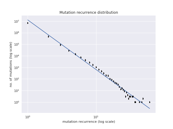
Finding the distribution of mutatios among genes
From the above example, we can see that, per nucleotide, the mutations can be considered essentially random. But, we can try to take a more coarse grained approach and quantify the mutations by gene so that it may be that the mutations divide randomly among all genes (in which case we may find almost all genes with the same number of mutations), or we may find that some genes have significantly more mutations than the rest.
This is how we may find out:
from collections import Counter
from ICGC_data_parser import SSM_Reader

# -- 1. Get the mutations count per gene

mutations_per_gene = Counter()

mutations = SSM_Reader(filename='data/ssm_sample.vcf')
consequences = mutations.subfield_parser('CONSEQUENCE')

for record in mutations:
    affected_genes = [c.gene_symbol for c in consequences(record) if c.gene_affected]
    mutations_per_gene.update(affected_genes)


# Show partial results
for gene,mutations in mutations_per_gene.most_common():
    print(f'{gene:<10}: {mutations}')
PCDH15    : 1651
RBFOX1    : 1041
CSMD1     : 979
DLG2      : 941
SPOCK3    : 929
DPP10     : 649
CTNND2    : 632
...
# -- 2. Now group by number of mutations

distribution = Counter(mutations_per_gene.values())
X    | NO. OF GENES WITH X MUTATIONS
----------------------------------------
1    | 8600
2    | 3624
3    | 1638
4    | 1403
6    | 1001
5    | 877
8    | 712
...
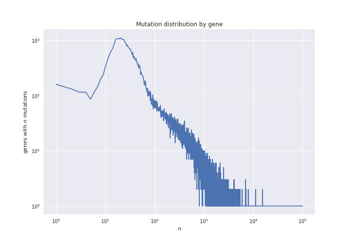
In the script mutations_distribution_genes.ipynb we can see how we
plot this data. For now, the resulting figure is the following:
But remember that genes have wildly varying lengths: 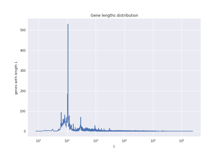
So, the distribution of mutations may be convoluted by the distribution of gene lengths. In order to smooth out this effect, we want to plot not the total number of mutations per gene, but the mutation density (the number of mutations normalized by the gene length).
To do this we need to check gene lengths, and the easiest way to do this
is via the Ensembl REST API, which we may use with the module
ensembl_rest. The following shows how to do this:
# In order to find out the length of the
# genes, we will use the Ensembl REST API.
import ensembl_rest
from itertools import islice

def chunks_of(iterable, size=10):
    """A generator that yields chunks of fixed size from the iterable."""
    iterator = iter(iterable)
    while True:
        next_ = list(islice(iterator, size))
        if next_:
            yield next_
        else:
            break
# ---


# -- 3. Normalize mutation counts by gene length


# Instantiate a client for communication with
# the Ensembl REST API.
client = ensembl_rest.EnsemblClient()


normalized_counts = Counter()
for gene_batch in chunks_of(mutations_per_gene, size=1000):
    # Get information of the genes
    gene_data = client.symbol_post('human',
                                   params={'symbols': gene_batch})

    gene_lengths = {gene: data['end'] - data['start'] + 1
                        for gene, data in gene_data.items()}

    # Get the normalization
    normalized_counts.update({
        gene: mutations_per_gene[gene] / gene_lengths[gene]
            for gene in gene_data
    })


# Show partial results
for gene,mutations in normalized_counts.most_common():
     print(f'{gene:<10}: {mutations}')
IGHD7-27  : 0.5454545454545454
IGKJ1     : 0.2894736842105263
IGKJ3     : 0.2894736842105263
IGKJ2     : 0.28205128205128205
SNORD112  : 0.18181818181818182
IGHJ3P    : 0.18
IGHJ5     : 0.16326530612244897
...
# -- 4. Aggregate by mutation density

normalized_distribution = Counter(normalized_counts.values())
X         | NO. OF GENES WITH X MUTATION DENSITY
----------------------------------------
0.9346%   | 112
0.9615%   | 33
0.9524%   | 26
0.9434%   | 23
1.6129%   | 20
1.8692%   | 20
0.9804%   | 19
1.2195%   | 19
...
Now we can plot this data. The code to do so is in the notebook
mutations_distribution_genes.ipynb. For now, the figure that results
is the following: 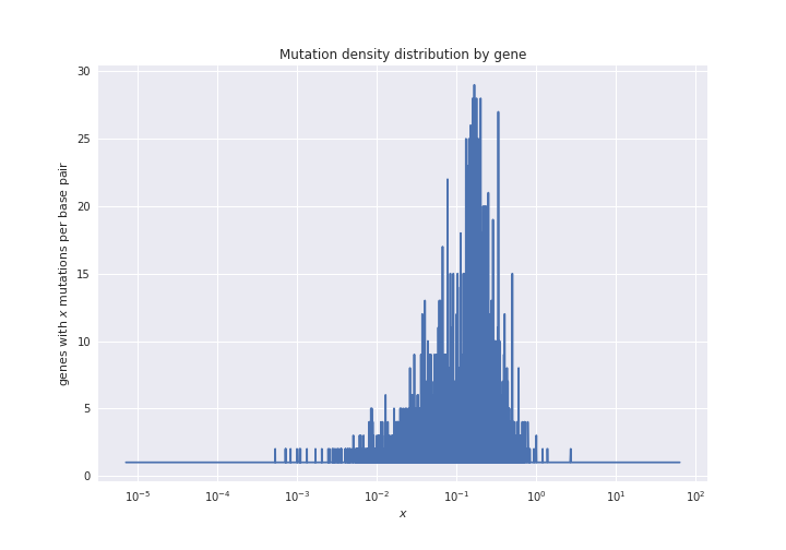
Plotting the mutation density in the chromosomes
The example notebook mutation_distribution_chroms.ipynb shows how to
plot the mutations distribution in the chromosomes. This is useful when
one wants to compare the variations among different projects. The
resulting figures are as the following one (with the chromosome and
centromere boundaries shown): 